One of the best places to get your feet wet with text mining is Twitter data. Though not as open as it used to be for developers, the Twitter API makes it incredibly easy to download large swaths of text from its public users, accompanied by substantial metadata. A treasure trove for data miners that is relatively easy to parse.
It’s also a great source of data for those studying the distribution of (mis)information via digital media. This is something I’ve been working on a lot lately, both in independent projects and in preparation for my courses on Digital Storytelling, Digital Studies, and The Internet. It’s amazing how much data you can get, and how detailed a picture it can paint about how citizens, voters, and activists find and disseminate information. Most recently, Bill Fitzgerald and I have begun discussing a project analyzing the distribution of (mis)information in extremist, so-called “alt-right” circles on Twitter, and comparing the language and information sources of left- and right-leaning communities on Twiter.
It turns out this is a really straightforward thing to do, thanks to Martin Hawksey’s TAGS (Twitter Archiving Google Sheet) and Julia Silge’s and David Robinson’s TidyText package for R. In what follows, I’ll walk through the process of setting up a TAGS archive, linking it to R, and mining it with TidyText (and other tools from the TidyVerse).
Setting up a TAGS archive
There are some excellent tools for interacting with the Twitter API directly, but if what you want is a regularly updating archive of tweets that you can repeatedly mine and analyze, TAGS is definitely the way to go. All you need is a Google account, a Twitter account, and a copy of Martin Hawksey’s Google Sheet, and you’re good to go. You don’t even need your own API key!
To set it up, make a copy of Martin’s TAGS sheet in your Google account. Then follow the instructions on the setup page to get up and running. After entering your search terms, I recommend setting it up to update every hour and making a one-off collection to start (“Run now!”). For more information on setting it up, check out Martin’s video:
Connecting your Google sheet with R
If you’re just planning on doing a one-time analysis of the tweets you archived, you can simply export your Google sheet as a CSV file (specifically, the Archive page), and read it into R with read.csv or read_csv. However, if you want to keep the archive updating over time and check on it regularly with R (or maybe even build a Shiny App that automatically updates analyses and visualizations for you!), you’ll need to publish your sheet to the web. Go to File >> Publish to the web... and publish the Archive page to the web as a CSV file. Be sure to check the box to automatically republish when changes are made. That way, when your Google sheet downloads new Twitter content each hour, it will also update the public CSV file.
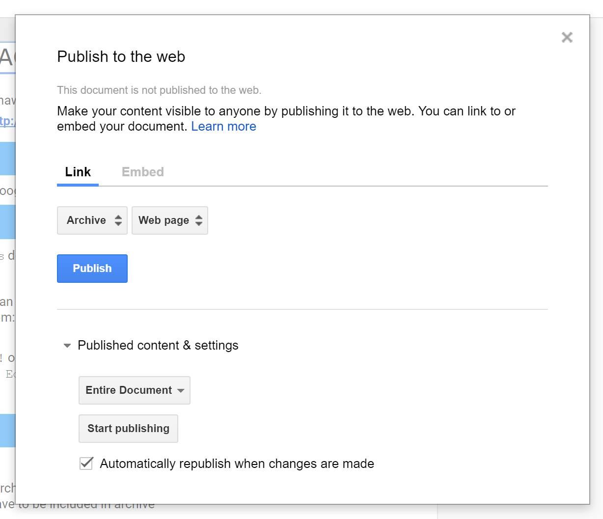
When you click Publish, it will give you a URL. Simply copy that URL and paste it into R:
tweets <- read_csv('https://docs.google.com/spreadsheets/d/your-archive-page-id-here',
                   col_types = 'ccccccccccccciiccc')
The col_types will ensure that the long, numeric ID numbers import as characters, rather than convert to (rounded) scientific notation.
Now you have your data, updated every hour, accessible to your R script!
Mining the tweets with TidyText (and dplyr and tidyr)
One of my favorite tools for text mining in R is TidyText. It was developed by a friend from grad school, Julia Silge, in collaboration with her (now) Stack Overflow colleague, David Robinson. It’s a great extension to the TidyVerse data wrangling suite. (Also, you should pre-order their new book, Text Mining with R: A Tidy Approach.)
Let’s walk through some of the things you can do with your Twitter archive using TidyText (and the TidyVerse in general). As an example, I’ll reference my growing collection of tweets with the hashtag #americafirst. (Note that though the tweets are technically public, I want to protect user privacy, so I won’t be linking to my Google sheet here or providing anything other than aggregate results. If you want, you can reproduce the study with the code, though it will return a later batch of tweets.)
First, load the necessary libraries, import the data from your Google sheet, and append an R-friendly date column.
library(tidyverse)
library(tidytext)
library(lubridate)
library(stringr)
library(httr)

google_sheet_csv <- '' #insert URL of published CSV file from TAGS archive Google sheet
tweets <- read_csv(google_sheet_csv,
                   col_types = 'ccccccccccccciiccc') %>%
  mutate(date = mdy(paste(substring(created_at, 5, 10), substring(created_at, 27 ,30))))

source_text <- '#americafirst'
minimum_occurrences <- 5 # minimum number of occurrences to include in output
This will give you a tibble (a tidy data frame) where each row is a tweet, and each column contains (meta)data for that tweet. I’ve also declared two variables that will help out in the parsing later.
To find the most frequent words, hashtags, or Twitter handles in the archive, we can pretty much lift the code out of Julia and David’s ebook:
reg_words <- "([^A-Za-z_\\d#@']|'(?![A-Za-z_\\d#@]))"
tidy_tweets <- tweets %>%
filter(!str_detect(text, "^RT")) %>%
mutate(text = str_replace_all(text, "https://t.co/[A-Za-z\\d]+|http://[A-Za-z\\d]+|&|<|>|RT|https", "")) %>%
unnest_tokens(word, text, token = "regex", pattern = reg_words) %>%
filter(!word %in% stop_words$word,
str_detect(word, "[a-z]"))
This snippet of code filters out any tweets whose text begins with RT (retweets; delete or comment out that line to keep retweets in), removes URLs and certain characters that signal something other than natural language text from the tweets, and tokenizes the tweets into words. That means splitting the text by spaces, removing punctuation, converting all letters to lower-case, etc., and then applying all of the metadata for the tweet to each individual word. A tweet with 10 words is a single record in the tweets data frame, but after tokenizing will result in 10 records in the new tidy_tweets data frame, each with a different word, but identical metadata. After tokenizing, we filter out any records where the word is contained in a list of stop words (a, an, the, of, etc.) or where the “word” contains no letters (i.e., raw numbers).
What’s unique about the way TidyText is tokenizing the Twitter data here is that it uses a regular expression to parse data in a Twitter-specific way. This regular expression includes all alphanumeric characters and the hash # and at-reply @ symbols. (Julia and David drop those in their ebook analyses, but I want to filter out all Twitter handles for privacy, as well as apply special analysis to hashtags, so I’m leaving them in.) It doesn’t always do this. For natural language, you can usually just tokenize by a pre-defined “word” concept, or n-gram. But this approach is necessary when parsing text that contains a lot of URLs and special symbols, as tweets do.
To find the most common words in this tweet corpus, we can use the following code to count occurrences of each unique word, filter out the most common (n > 150, in this case), and order them most to least frequent.
tidy_tweets %>%
  count(word, sort=TRUE) %>%
  filter(n > 150) %>%
  mutate(word = reorder(word, n))
This produces:
# A tibble: 31 × 2
               word     n
             <fctr> <int>
1     #americafirst  5593
2             #maga  2530
3            #trump   821
4            @potus   742
5  @realdonaldtrump   741
6       #trumptrain   666
7             trump   503
8               #2a   457
9    #draintheswamp   432
10    #buildthewall   408
# ... with 21 more rows
All hashtags and Twitter handles! Let’s see what’s most common if we omit hashtags and handles:
tidy_tweets %>%
count(word, sort=TRUE) %>%
filter(substr(word, 1, 1) != '#', # omit hashtags
substr(word, 1, 1) != '@') %>% # omit Twitter handles
mutate(word = reorder(word, n))
# A tibble: 6,533 × 2
word n
<fctr> <int>
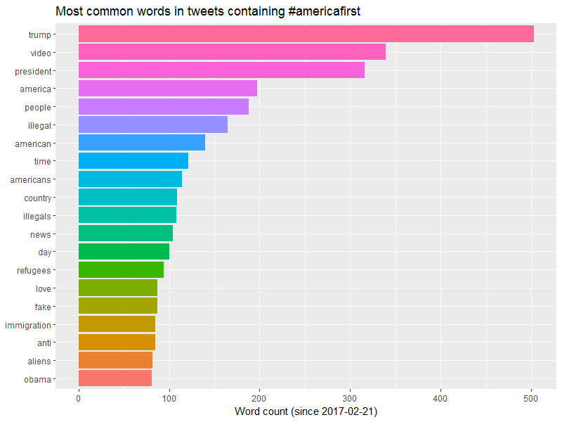
1 trump 503
2 video 339
3 president 316
4 america 197
5 people 188
6 illegal 165
7 american 140
8 time 121
9 americans 114
10 country 109
# ... with 6,523 more rows
To make this count into a new data frame (to view the whole thing or save to a file), just assign it to a variable.
word_count <- tidy_tweets %>%
  count(word, sort=TRUE) %>%
  filter(substr(word, 1, 1) != '#', # omit hashtags
         substr(word, 1, 1) != '@') %>% # omit Twitter handles
  mutate(word = reorder(word, n))
Or visualize it with ggplot2 (part of the TidyVerse meta-package).
tidy_tweets %>%
  count(word, sort=TRUE) %>%
  filter(substr(word, 1, 1) != '#', # omit hashtags
         substr(word, 1, 1) != '@', # omit Twitter handles
         n > 80) %>% # only most common words
  mutate(word = reorder(word, n)) %>%
  ggplot(aes(word, n, fill = word)) +
  geom_bar(stat = 'identity') +
  xlab(NULL) +
  ylab(paste('Word count (since ',
             min_date,
             ')', sep = '')) +
  ggtitle(paste('Most common words in tweets containing', source_text)) +
  theme(legend.position="none") +
  coord_flip()
Often times, looking for the most common bigrams (two-word phrases) is more instructive than individual words. Using TidyText to do this with Twitter data is a bit more complicated, as you need to parse by regex, rather than use the built-in n-gram option. Julia and David don’t give an example in their ebook, but it’s not too hard. We simply tokenize by regex like before, use dplyr’s lead() function to append the following word to each record, and then unite() the two into a single bigram (assuming they both belong to the same tweet). Here’s how to do that, as well as to remove bigrams containing hashtags, Twitter handles, raw numbers, stop words.
tidy_bigrams <- tweets %>%
filter(!str_detect(text, "^RT")) %>%
mutate(text = str_replace_all(text, "https://t.co/[A-Za-z\\d]+|http://[A-Za-z\\d]+|&|<|>|RT|https", "")) %>%
unnest_tokens(word, text, token = "regex", pattern = reg_words) %>%
mutate(next_word = lead(word)) %>%
filter(!word %in% stop_words$word, # remove stop words
!next_word %in% stop_words$word, # remove stop words
substr(word, 1, 1) != '@', # remove user handles to protect privacy
substr(next_word, 1, 1) != '@', # remove user handles to protect privacy
substr(word, 1, 1) != '#', # remove hashtags
substr(next_word, 1, 1) != '#',
str_detect(word, "[a-z]"), # remove words containing ony numbers or symbols
str_detect(next_word, "[a-z]")) %>% # remove words containing ony numbers or symbols
filter(id_str == lead(id_str)) %>% # needed to ensure bigrams to cross from one tweet into the next
unite(bigram, word, next_word, sep = ' ') %>%
select(bigram, from_user, date, id_str, user_followers_count, user_friends_count, user_location)
Now we can count and sort the bigrams.
tidy_bigrams %>%
  count(bigram, sort=TRUE) %>%
  mutate(bigram = reorder(bigram, n))
This gives us:
# A tibble: 4,857 × 2
bigram n
<fctr> <int>
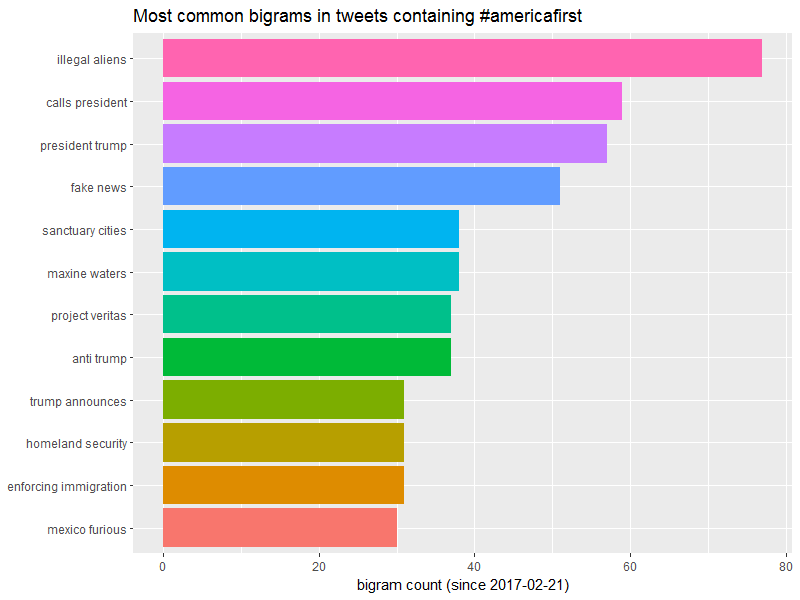
1 illegal aliens 77
2 calls president 59
3 president trump 57
4 fake news 51
5 maxine waters 38
6 sanctuary cities 38
7 anti trump 37
8 project veritas 37
9 enforcing immigration 31
10 homeland security 31
# ... with 4,847 more rows
And we can plot it like before.
tidy_bigrams %>%
  count(bigram, sort=TRUE) %>%
  filter(n >= 30) %>%
  mutate(bigram = reorder(bigram, n)) %>%
  ggplot(aes(bigram, n, fill = bigram)) +
  geom_bar(stat = 'identity') +
  xlab(NULL) +
  ylab(paste('bigram count (since ',
             min_date,
             ')', sep = '')) +
  ggtitle(paste('Most common bigrams in tweets containing', source_text)) +
  theme(legend.position="none") +
  coord_flip()
We can do a lot with this word and bigram data, as Julia and David’s ebook demonstrate. We can produce a network analysis of words (essentially a 2D visualization of a Markov model; we could also do this with user data), we can compare word or bigram frequency with another Twitter corpus, and we could search for the most common hashtags and handles in the corpus to find other terms to add to the search that generates the TAGS archive.
One thing Bill and I want to look at, though, is where some of the people using these hashtags are getting the information that they are sharing. In other words, we want to access only the URLs we filtered out at the beginning, and use them to find out which articles and which domains appear the most often. So let’s go back to the beginning and do that.
We don’t need to reimport the data, as the tweets tibble still contains the raw imported tweets with all the metadata. We just have to re-parse the tweets.
reg <- "([^A-Za-z_\\d#@:/']|'(?![A-Za-z_\\d#@:/]))"
urls_temp <- tweets %>%
unnest_tokens(word, text, token = "regex", pattern = reg, to_lower = FALSE) %>%
mutate(word = str_replace_all(word, "https|//t|http|&|<|>", ""),
word = str_replace_all(word, "co/", "https://t.co/")) %>%
select(word) %>%
filter(grepl('https://t.co/', word, fixed = TRUE)) %>%
count(word, sort=TRUE) %>%
mutate(word = reorder(word, n))
Note the differences in this parse code: the regular expression now includes the forward slash. Without it, we’d lose the URL strings. Also note the to_lower = FALSE option in unnest_tokens. All URLs returned by the Twitter API use the t.co URL shortener, which uses case-sensitive strings for their URLs. Without to_lower = FALSE, TidyText would make everything lower-case, and our URLs would be useless. The first mutate command should look familiar, except that it no longer removes whole URLs that contain https://t.co. Instead, it removes only the https. What we’re left with, at this point, is a bunch of “words” of the form co/juMbl3OfCh@ract3r$. We want to re-construct these into full URLs, which the next line does for us. Then we remove all metadata, and then all “words” that don’t contain https://t.co/. This will leave us only with t.co shortened URLs, count them, and sort them by frequency, saved in a new data frame urls_temp.
But a bunch of t.co URLs isn’t very helpful. We want the targets they point to! Thankfully, Hadley Wickham’s httr package can do that for us! First, let’s limit ourselves to the most common URLs. (Remember that minimum_occurrences = 5 we set at the beginning? That will save us a lot of processing time, while only skipping over URLs that contribute little to the corpus data.)
urls_common <- urls_temp %>%
  filter(n >= minimum_occurrences) %>%
  mutate(source_url = as.character(word)) %>%
  select(source_url, count = n)
Now we use httr to obtain the target URLs for those t.co URLs in the corpus that occur at least five times, and return an HTTP status code (so we can filter out any broken links). This will take some time, especially for a large corpus. If you regularly return to a large, growing corpus, I recommend saving the results to a CSV file, and then importing that CSV file and using anti_join() so you can limit your GET requests only to URLs you haven’t already tracked down.
url <- t(sapply(urls_common$source_url, GET)) %>%
  as_tibble() %>%
  select(url, status_code)
Then we can bind those results to the original URLs and their frequency count, and filter out any 404 statuses (page not found), and any URLs that point back to Twitter (like quoted tweets). Of course, you can leave those in if it makes sense for your project.
url_list <- cbind(urls_common, unnest(url)) %>%
  as_tibble() %>%
  select(url, count, status_code) %>%
  filter(status_code != 404,
         url != 'https://t.co/',
         !grepl('https://twitter.com/', url))
Now we have a list of URLs, sorted by how frequently they occur in our corpus! A great way to identify the (mis)information sources in an online community.
If it’s not articles but sites we’re after, we can just parse the URL character string to get to the root domain of each URL and count those instead.
# extract domains from URLs
extract_domain <- function(url) {
  return(gsub('www.', '', unlist(strsplit(unlist(strsplit(as.character(url), '//'))[2], '/'))[1]))
}

# count the frequency of a domain's occurrence in the most frequent URL list
domain_list <- url_list %>%
  mutate(domain = mapply(extract_domain, url)) %>%
  group_by(domain) %>%
  summarize(domain_count = sum(count)) %>%
  arrange(desc(domain_count))
That first function is really messy! It’s simply splitting the URL by // and taking everything to the right of that, then splitting it by / and taking everything to the left of the first slash, then dropping www., if present.
This gives us a very interesting mix of domains found in the #americafirst tweets.
# A tibble: 33 × 2
                     domain domain_count
                      <chr>        <int>
1             breitbart.com          446
2            patriotpost.us          139
3          pamelageller.com          137
4    NewsUnitedStates.co.vu          105
5               youtube.com          101
6          americaspaper.ml           69
7            USATrump.co.vu           34
8  overpassesforamerica.com           30
9               foxnews.com           26
10           whitehouse.gov           25
# ... with 23 more rows
Which we can also plot.
domain_list %>%
  mutate(domain = reorder(domain, domain_count)) %>%
  ggplot(aes(domain, domain_count, fill = domain)) +
  geom_bar(stat = 'identity') +
  xlab(NULL) +
  ylab(paste('domain count (since ',
             min_date,
             ')', sep = '')) +
  ggtitle(paste('Most common domains in tweets containing', source_text)) +
  theme(legend.position="none") +
  coord_flip()
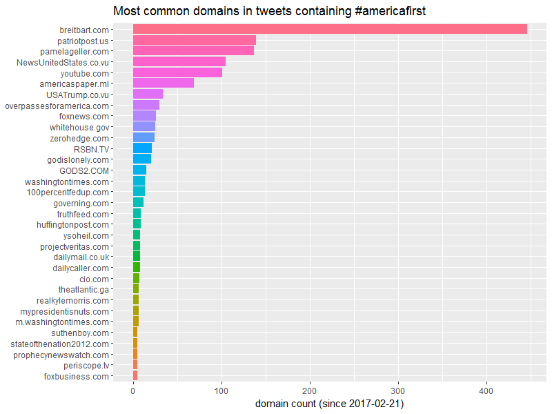
And if you follow further redirects for root domains, guess what you find! Those sites supposedly from Mali and Vanuatu? They redirect to adf.ly, whose motto is “Get paid to share your links on the Internet!” Add them together, and they’re the second-highest frequency of the domains in this corpus. I smell something fishy. But that’s for another day…
On GitHub
I’ve put all of this code (and a little more) in a GitHub repository, which I will continue to expand as time permits and my projects progress. Feel free to download it, test it out, and even send a pull request if you add some cool functionality to it!
Happy Twitter mining!
Header image by Pixabay.